Style transfer was first introduced by Aaron Hertzmann's classic paper on Image Analogies from SIGGRAPH 2001. More recently deep learning got applied to this problem in Leon Gatys paper "A Neural Algorithm of Artistic Style" which has led to a resurgence of work in this area. There are a few very good tutorials on this subject which the author will turn you towards for implementing Gatys' style transfer algorithm. Here are a couple
• Harish Narayanan's Convolutional neural networks for artistic style transfer, or • LogO - Implementing of a Neural Algorithm of Artistic Style
Both of these blogs explain Gatys' paper and my blog entry is about understanding the nitty gritty of these style transfer algorithms in the context of tensorflow.
High Level Problem
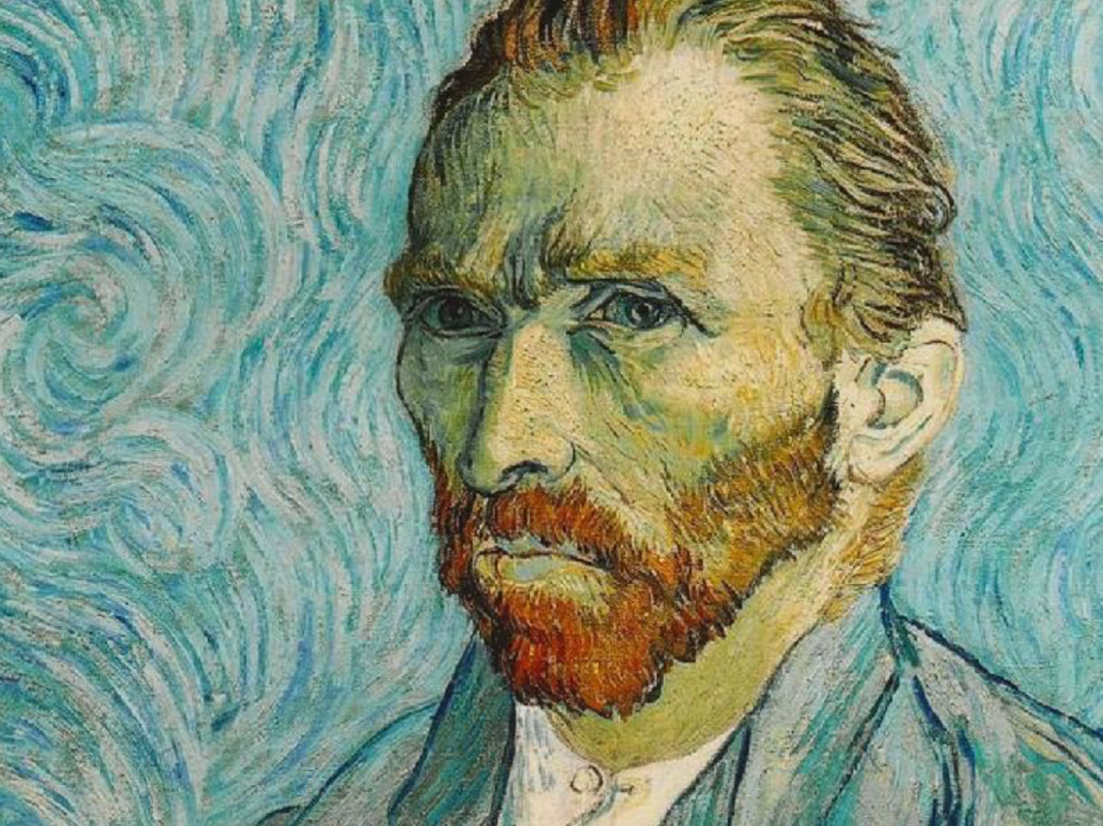
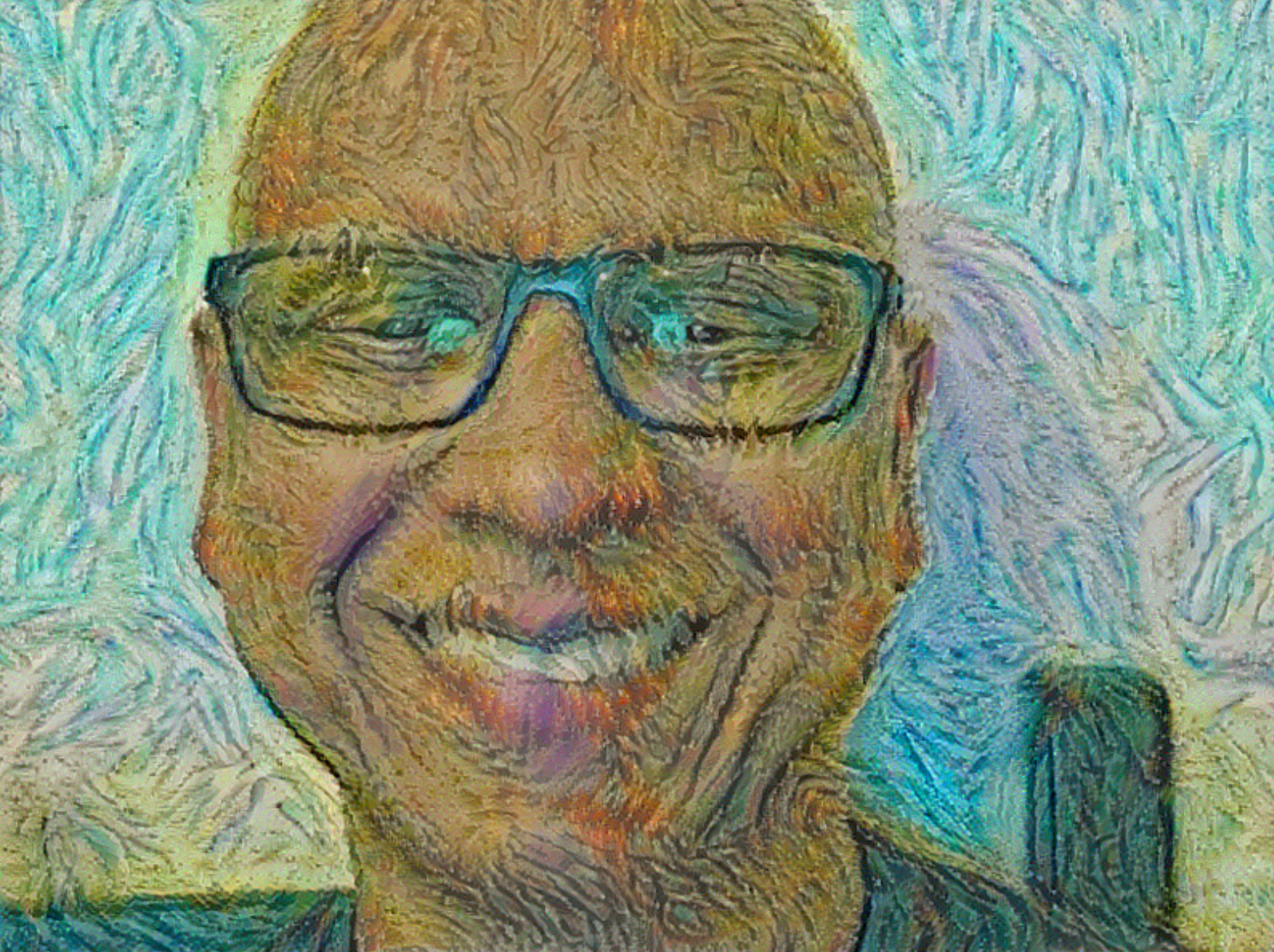
Style Transfer is applying the style from one image to the content of another.

Prior Knowledge
VGG-19 is a 19 layer neural network created by Karen Simonyan and Andrew Zisserman (Very Deep Convolutional Networks for Large-Scale Image Recognition). The neural networks takes as an input an image of size 224 x 224 × 3 and outputs a classification vector that can classify the image as one of a thousand different objects.
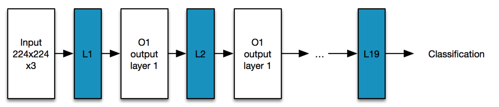
So, if we feed an image Ai to this network then the
- the output will be a classification of the image e.g. whether it is a house or a train
- the activation at each of hidden layers (blue) are L1(Ai), L2(Ai).. And L19(Ai). The activation at each layer represents a feature of the image that the network has learnt.
Idea
So, if the distance between activations from two images A1 and A2 is small ((L1(A1), L2(A1), L3(A1)... L19(A1)), L1(A2), L2(A2), L3(A2)... L19(A2))) then we know that the two images are similar (and probably the same).
Similarly if the distance between the gram matrices of the activations from A1 and A2 is small then the two images are similar in style. For now assume that this is so.
So, we define two costs which capture content similarity and style similarity and setup an optimization problem to minimize the two. When the cost is minimized, we have generated an image that has the content from the first and the style from the 2nd. Note that we wont focus too much on explaining this part since it has been explained well in the Gatys paper.
The Genius is in the Details
For the rest of this post, I will assume that you get the code from logO's implementation and code pieces refer to the art.py file from his work.
If the Neural Network takes a 224x224x3 input, then how can we use it to input an image that is 600x800.
In a CNN (specifically VGG-19) there are a few different types of layers convolution_2D, relu, maxpool and fully connected (FC). If the VGG-19 is modified to handle a 600x800 input then.
-
In the layers of the network prior to FC layers each layer will be of a different size but convolution filters are scale independent so the previously learnt weights will continue to work. So for example the first hidden layer after pooling is 112x112x64 in the classic VGG-19 but in our example it will be 400x300x64. Even though the size of the layer is larger the same pre-trained weights for the convolution filters will work and activate on same features.
-
The fully connected layers will need different number of weights and retraining, but we will not use that part of the network.
If the output of the VGG-19 network is 1x1x1000 then how do we use it to compute an image that is 600x800x3?
We already know that we wont be using the standard VGG-19 network, specially the fully connected layers. Let me show you how the optimization problem is set up in such a way that solving for the generated image (see red/blue/green image below) minimizes the style and content cost.
Creation of the neural network
(excerpt from the art.py file)
graph = {}
graphl 'input'] = tf. Variable(np.zeros ((1, IMAGE_HEIGHT, IMAGE_WIDTH, COLOR_CHANNELS)),
graph['conv1_1'] =_conv2d_relu(graph['input'], 0, 'conv1_1')
graph['conv1_2'] =_conv2d_relu(graph['conv1_1'], 2, 'conv1_2')
graph ['avgpool1'] =_avgpool(graph['conv1_2'])
graph['conv2_1'] =_conv2d_relu(graph['avgpool1'], 5, 'conv2 _1')
graph['conv2_2'] =_conv2d_relu(graph['conv2_1'], 7, 'conv2_2')
graph['avgpoo12'] =_avgpool(graph['conv2_2'])
graphl'conv3_1'] =_conv2d_relu(graphl'avgpool2'], 10, 'conv3 _1')
graph ['conv3_2'] = _conv2d. _relu(graphI'conv3_1'], 12, 'conv3 _2')
graph['conv3_3'] =_conv2d_relu(graph['conv3_2'], 14, 'conv3_3')
graph['conv3_4'] =_conv2d_relu(graph['conv3_3'], 16, 'conv3_4')
graph ['avgpoo13'] =_avgpool(graph|'conv3_4'])
graph['conv4_1'] =_conv2d_relu(graph['avgpool3'], 19, 'conv4_1') 'conv4_1')
graph['conv4_2'] =_conv2d_relu(graph['conv4_1'], 21, 'conv4_2')
graph['conv4_3'] =_conv2d_relu(graph['conv4_2'], 23, 'conv4_3')
graph['conv4_4'] =_conv2d_relu(graph['conv4_3'], 25, 'conv4_4')
graph l'avgpoo14'] =_avgpool(graph['conv4_4'])
graph['conv5_1'] =_conv2d_relu(graph['avgpool4'], 28, 'conv5_1') 'conv5_1')
graphl 'conv5_2'] =_conv2d_relu(graph['conv5_1'], 30, 'conv5_2') 'conv5_2')
graph['conv5_3'] =_conv2d_relu(graph['conv5_2'], 32, 'conv5_3') 'conv5_3')
graph['conv5_4'] =_conv2d_relu(graph['conv5_3'], 34, 'conv5_4') "conv5_4')
graph ['avgpool5'] =_avgpool(graph['conv5_4'])
If you study this code then you learn...
- The neural network is setup as a tensorflow computational graph with only one "variable" layer which is the first layer. None of the entries in the rest of the tree are "variables". The output of any of these layers can be computed given the input but the weights of each of these layers is fixed at this point.
- graph['input'] = tf.Variable(np.zeros((1, IMAGE_HEIGHT, IMAGE_WIDTH, COLOR_CHANNELS)), dtype = 'float32'). The size of graph['input'] is IMAGE_HEIGHT, IMAGE_WIDTH, COLOR_CHANNELS which can be set to 600 × 800 × 3.
- sess.run(graph['input'].assign(content_image). is used to initialize the first layer of the CNN with an image.
In tensorflow variables are the only objects whose values can change when optimization is run. Now let us see how to setup the optimization problem.
Setting up the Optimization Problem
Let us assume that there are two functions content_cost and style_cost that we have to minimize, both of them take activations of two neural networks' layers as input.
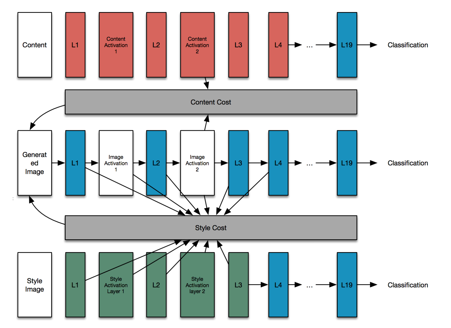
In this set up the neural network is instanciated three times but only the middle one is used for the optimization. In art.py let us look at the definition of content_loss_func carefully.
def content_loss_func(sess, model):
   """
   Content loss function as defined in the paper.
   """
   def _content_loss(p, x):
      # N is the number of filters (at layer l).
      N = p.shape[3]
      # M is the height times the width of the feature map (at layer l).
      M = p.shape[1] * p.shape[2]
      # Interestingly, the paper uses this form instead:
      #
      # 0.5 * tf.reduce_sum(tf.pow(x - p, 2))
      #
      # But this form is very slow in "painting" and thus could be missing
      # out some constants (from what I see in other source code), so I'll
      # replicate the same normalization constant as used in style loss.
      return (1 / (4 * N * M)) * tf.reduce_sum(tf.pow(x - p, 2))
return _content_loss(sess.run(model['conv4_2']), model['conv4_2'])
If you look at the last line of the function then _content_loss is compared between sess.run(model['conv4_2']) and model['conv4_2']. And the difference between the first and the second is that the one where the session has been executed, the value is the instantiated value of the hidden layer (top layer, red). Here the links between the previous layers of the neural network are no longer valid. So, even though in the code it looks like the model is still active, it is really the values which are being used. In fact the type of the red layers after sess.run is of type numpy.darray and not tensorflow. Same with the green squares in the 3rd network.
So, for all intents and purposes the top and bottom neural network may not have existed and we are just optimizing for the only variable in the graph which is the generated image (see Figure).
To make this further clear, the types of the blue layers is a tensorflow ('tensorflow.python.framework.ops.Tensor') whereas the type of the red / green layers is a numpy array. ('numpy.ndarray')
How to Compute a Neural Network only to a certain Point?
For a newcomer, it is sometimes not clear how to compute a neural network only to a certain point and not all the way to the final output. So, for example for the figure above the network in blue what if I only want the activations in layer L4.
There are two use cases for this:
- Connecting up the tensor-flow graph to create a new larger graph which will eventually be used for computation. In this case you will use graph['conv2_1'] to connect up the network. In our example when we constructed the network we had created a dictionary of node names for easy reference. This is how the blue network got connected in this particular example.
- Finding the actual value of the activation layer for a specific input. There are two steps in this use case:
     sess.run(graph['input'].assign(content_image))
     activation_layer = sess.run(graph['conv2_1'])
The first line initializes the variable to a particular value (this step can be omitted if the variable already has certain value) and the second line executes the tensorflow graph to get the value of the layer of type numpy.darray. It is no longer connected to the rest of the network. This is how the red and the green network got connected in this example. Note that the bottom layers in green (or the top layers in red) are not connected to each other.